Using Additional Arguments of `Quandl()` Function

The function call Quandl("GOOG/FRA_BMW") without any additional arguments returns a data frame with six columns, namely 'Date', 'Open', 'High', 'Low', 'Close' and 'Volume' for all available dates. Furthermore, the data frame is returned in descending order. Our R object bmw ranges from 2011-01-03 to 2015-09-18.

If you want to truncate your time series the two arguments start_date and end_date of the Quandl function can be used.

In a next step, we only want to download the BMW data for 2014 and we want the ordering of the data to change from descending to ascending. Both arguments start_date and end_date have to be in the format 'yyyy-mm-dd'.

> bmw_2014 <- Quandl("GOOG/FRA_BMW",
+                    start_date = "2014-01-01", end_date = "2014-12-31",
+                    order = "asc")

> str(bmw_2014)

'data.frame':    252 obs. of  6 variables:
 $ Date  : Date, format: "2014-01-02" "2014-01-03" ...
 $ Open  : num  85.3 83.5 84 83.1 83.9 ...
 $ High  : num  86 84.4 84.3 84 84.6 ...
 $ Low   : num  83.5 83.5 82.9 82.5 83.8 ...
 $ Close : num  83.5 84 83.2 83.6 84.5 ...
 $ Volume: num  14509 3476 4932 5129 6477 ...
 - attr(*, "freq")= chr "daily"

> head(bmw_2014)

        Date  Open  High   Low Close Volume
1 2014-01-02 85.28 86.01 83.50 83.54  14509
2 2014-01-03 83.50 84.40 83.50 84.03   3476
3 2014-01-06 84.05 84.33 82.86 83.19   4932
4 2014-01-07 83.10 84.01 82.47 83.60   5129
5 2014-01-08 83.90 84.64 83.83 84.46   6477
6 2014-01-09 84.55 85.11 83.72 84.18   7907

Comparing both R objects bmw and bmw_2014 we have reduced the observations for each of the columns from 1197 to 252. The dates we have data for range from 2014-01-02 to 2014-12-30.

By default, Quandl() returns data as class data.frame which is not the best output type when dealing with time series.

Quandl() offers several different output classes,

data.frame
ts
zoo
xts
timeSeries,

which can be chosen with type argument.

An overview about the different classes and corresponding packages can be found in the CRAN Task View: Time Series Analysis or in the pdf Working with Financial Time Series Data in R written by Eric Zivot.

To get an output with class zoo the function call would look like this:

> bmw_2014_zoo <- Quandl("GOOG/FRA_BMW",
+                        start_date = "2014-01-01", end_date = "2014-12-31",
+                        order = "asc", type = "zoo")

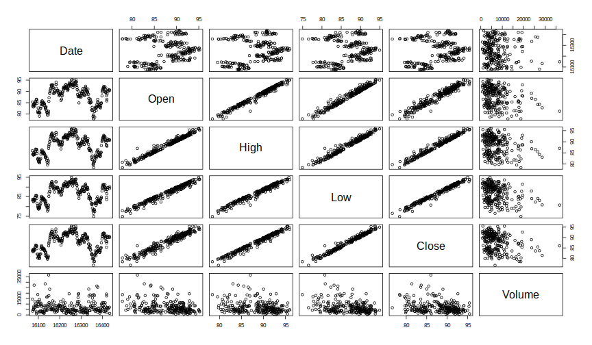
Let's have a look at what the standard plot function produces for both classes.

> plot(bmw_2014)

plot of chunk plotcomp

> plot(bmw_2014_zoo)

plot of chunk plotcomp

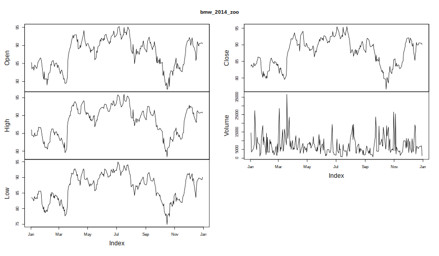
First call produces a scatterplot matrix whereas the columns of the data frame are plotted against each other. Second call returns plotted time series for each column which is more appropriate for our data.

The reason for this behavior is that 'plot' function checks the classes of the objects to be visualized. So under the hood for an object with class 'data.frame' the function 'plot.data.frame' from package graphics is used and for objects with class 'zoo' the 'plot.zoo' function in package zoo.

Now we have data on a daily basis but Quandl() offers several more choices like,

weekly
monthly
quarterly
annual,

which can be achived using the collapse argument. By collapsing a daily dataset to weekly, you will get a sample of the original dataset where the observation for each week is the last data point available for that week.

To download weekly data of 2014 for BMW equity from Frankfurt Stock Exchange the function call would be

> bmw_2014_zoo_weekly <- Quandl("GOOG/FRA_BMW",
+                               start_date = "2014-01-01", end_date = "2014-12-31",
+                               order = "asc", type = "zoo", collapse = "weekly")

> str(bmw_2014_zoo_weekly)

'zoo' series from 2014-01-05 to 2015-01-04
  Data: num [1:53, 1:5] 83.5 84.3 85.6 84.7 80.6 ...
 - attr(*, "dimnames")=List of 2
  ..$ : NULL
  ..$ : chr [1:5] "Open" "High" "Low" "Close" ...
  Index:  Date[1:53], format: "2014-01-05" "2014-01-12" "2014-01-19" "2014-01-26" ...

> head(bmw_2014_zoo_weekly)

            Open  High   Low Close Volume
2014-01-05 83.50 84.40 83.50 84.03   3476
2014-01-12 84.26 84.26 83.14 83.65  27281
2014-01-19 85.57 86.73 85.56 86.34   8630
2014-01-26 84.72 84.75 81.69 81.97  12149
2014-02-02 80.62 80.98 78.66 80.72   9208
2014-02-09 82.15 82.15 81.08 82.07   3565

It is also possible to apply various transformations to the data.

Suppose we have a time series with time stamps $i = 0, \ldots, I$, where $x_0$ refers to the starting date for the API call specified by start_date and $x_I$ refers to the end point specified by end_date.

Possible values for the transform argument are

none: leave the data as it is
diff: shows the row - on - row change; $x^{*}_i = x_i - x_{i-1}$
rdiff: shows the relative row - on - row change; $x^{*}_i = \dfrac{(x_i - x_{i-1})}{x_{i-1}}$
normalize: set starting value at 100; $x^{*}_i = \dfrac{x_i}{x_0} \cdot 100$
cumul: shows the cumulative sum; $x^{*}_i = x_i + x_{i-1} + x_{i-2} + \ldots + x_0$
rdiff_from: shows ratio between the latest point and an earlier point; $x^{*}_i = \dfrac{(x_I - x_{i})}{x_{i}}$

Furthermore, you can select single columns of the data. If we want the returns of the closing prices (fourth column) of 2014 for BMW we have to call the Quandl function like this

> bmw_2014_returns <- Quandl("GOOG/FRA_BMW.4",
+                            start_date = "2014-01-01", end_date = "2014-12-31",
+                            order = "asc", type = "zoo", transform = "rdiff")
> 
> head(bmw_2014_returns)

  2014-01-03   2014-01-06   2014-01-07   2014-01-08   2014-01-09 
 0.005865454 -0.009996430  0.004928477  0.010287081 -0.003315179 
  2014-01-10 
-0.006296032

Finally, you can also get meta data. The only thing needed to receive this information is to switch the meta argument from FALSE to TRUE.

> bmw_2014_zoo_meta <- Quandl("GOOG/FRA_BMW",
+                             start_date = "2014-01-01", end_date = "2014-12-31",
+                             order = "asc", type = "zoo", meta = TRUE)
> str(bmw_2014_zoo_meta)

'zoo' series from 2014-01-02 to 2014-12-30
  Data: num [1:252, 1:5] 85.3 83.5 84 83.1 83.9 ...
 - attr(*, "dimnames")=List of 2
  ..$ : NULL
  ..$ : chr [1:5] "Open" "High" "Low" "Close" ...
 - attr(*, "meta")=List of 20
  ..$ id                   : int 6269390
  ..$ dataset_code         : chr "FRA_BMW"
  ..$ database_code        : chr "GOOG"
  ..$ name                 : chr "Bayerische Motoren Werke AG (BMW)"
  ..$ description          : chr "Bayerische Motoren Werke AG is a German holding company and automobile manufacturer that focuses on the automobile and motorcyc"| __truncated__
  ..$ refreshed_at         : chr "2015-09-19T04:20:43.065Z"
  ..$ newest_available_date: chr "2015-09-18"
  ..$ oldest_available_date: chr "2011-01-03"
  ..$ column_names         : chr [1:6] "Date" "Open" "High" "Low" ...
  ..$ frequency            : chr "daily"
  ..$ type                 : chr "Time Series"
  ..$ premium              : logi FALSE
  ..$ limit                : NULL
  ..$ transform            : NULL
  ..$ column_index         : NULL
  ..$ start_date           : chr "2014-01-01"
  ..$ end_date             : chr "2014-12-31"
  ..$ collapse             : NULL
  ..$ order                : chr "asc"
  ..$ database_id          : int 393
  Index:  Date[1:252], format: "2014-01-02" "2014-01-03" "2014-01-06" "2014-01-07" ...

The meta attribute of the object bmw_2014_zoo_meta is a list with 20 entries, such as frequency, name, description etc. . Assuming that we are interested in an extended description of BMW we can get this with

> attr(bmw_2014_zoo_meta,"meta")$description

Bayerische Motoren Werke AG is a German holding company and automobile manufacturer that 
focuses on the automobile and motorcycle markets. It divides its activities into the
three main segments: Automobiles, Motorcycles and Financial Services.
It owns three brands: BMW, MINI and Rolls-Royce. Its BMW automobile range
encompasses the 1 Series, including three-door, five-door, coupe and convertible models;
the 3 Series, including sedan, touring, coupe and convertible models;
the 5 Series, available in sedan and touring models;
the 6 Series, available as a coupe or convertible;
the 7 Series large sedan; the Z4 roadster and coupe;
the sports utility vehicles, X3, X5 and X6 and M models, such as M3, M5 and M6.
It also offers cars under the MINI brand and motorcycles under the BMW brand.
The Rolls-Royce brand offers three luxury cars, Phantom, Coupe and Ghost.
It has producing, assembly, service and sales subsidiaries throughout the world.
In January 2013, it sold its Husqvarna brand.

Using Additional Arguments of Quandl() Function

Using Additional Arguments of `Quandl()` Function